Tai Xiang's Random Projects

So a little while back we talked about LSTMs and how they were so much better than that mishmash of classifiers we used to create a voted classifier. We talked about how the LSTM was so much smarter than those other deep learning models and neural nets and how it was well suited for text processing.

Well apparently the LSTM is kind of stupid as well.

Ok, that’s an over-exaggeration. Maybe ‘not the smartest guy in the room’ is a better phrase to use. Someone else has claimed that title.

Prior to 2017, the LSTM would’ve handily nabbed that crown, but nowadays, the Transformer is the new state-of-the-art model for many text processing tasks. Although you’ve probably got images of robots whizzing about as over-the-top explosions rock the screen and an abundance of American flags are shoved in your face, you’re going to want to push those down. We’re going to be talking about something that is much more intelligently put together and doesn’t tarnish memories of your childhood.

The structure of the Transformer model is quite different from that of the LSTM. The LSTM RNN model is composed of a bunch of LSTM units, each with a cell, an input gate, an output gate, and a forget gate. Each of these gates play a role in supervising how information flows through the cell and is distributed over time. Since these LSTM units are all linked together, the output of the previous LSTM unit will be taken in as the input of the next one, and thus earlier learned information is passed from one unit to the next, which allows the LSTM to retain past information. However, the issue with this is each unit can only be dependent on the unit before it. The 5th LSTM won’t be able to see what the 3rd LSTM unit learned; it can only get the 4th units interpretation of the 3rd unit. Thus in order for the 5th unit to actually become active, the 4th unit must have finished processing and have created an output first. This makes the LSTM a sequential model. It goes from LSTM unit 1 to unit 2 to unit 3 to unit 4, with each preceding unit having to wait for the one before it to finish up before it can begin. Thus when we pass the LSTM a sentence such as “The dog runs through the forest.”, each word gets passed in sequentially aka one at a time. First ‘the’, then ‘dog’, then ‘run’, and so on and so forth. As a result, LSTMs take a long time to train as they are unable to utilize the powerful parallel computational abilities most modern GPUs provide.

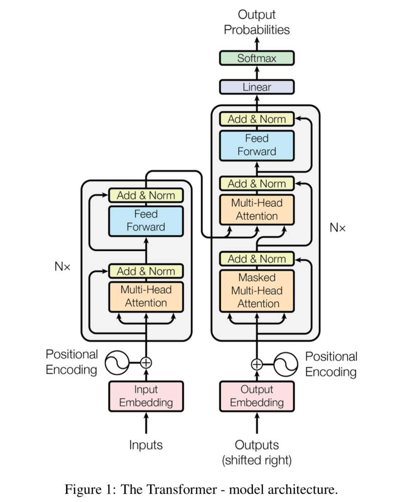
The Transformer scraps this sequential structure. Let’s take a dive into the architecture of the Transformers and see what makes it so interesting. Here’s what it looks like:

To understand the architecture of the Transformer, we must first designate a task we wish to complete. Let’s say we want to take the sentence “The dog runs through the forest.” and have our model generate a sentence that would logically follow it.

First, we take a peek at the encoder of our Transformer model, which is shown on the left of the model where the inputs go in. Viewing it from the perspective of natural language processing, the encoder of the model designates how our chunk of human text is converted into a model-readable representation, as these models only take in numbers and vectors as input (an example of this is discussed in the LSTM post). Earlier in the LSTM post I stated that these models don’t take in text, they take in text that have been encoded into vectors known as word embeddings or into some form of integer representation. That is an example of the encoding process. The Transformer’s encoder allows it to process text in parallel. It doesn’t have to take in each word sequentially, it can simply eat up the whole entire phrase.

To do this, the Transformer makes use of something known as a positional encoder and an attention mechanism. The positional encoder (which is represented by a vector) designates where in the sentence each word is positioned. For the phrase “The dog runs through the forest”, the word ‘The’ will have a positional encoder designating it to be in position one, while the word ‘dog’ will have a positional encoder designating it to be in position two, and so on and so forth.

Let’s look at our sentence “The dog runs through the forest” and say that hypothetically the word ‘dog’ is represented by the word embedding [1 32 12 43]. Now, suppose we add on the positional encoding (position two) to the word ‘dog’. The word embedding now becomes [2 44 23 52], with that change in value of the vector designating it to be in position two. If we vectorize all the text in our sentence and then apply our positional encodings, we now have a bunch of vectors that contains information that designate what each word is and where it goes in the sentence. Now we don’t have to pass each word into the model one at a time to retain order.

The exact equation that is used to calculate the positional encoder as well as all the technical bits and pieces of the Transformer architecture can be found in the paper “Attention is all you Need”.

Another interesting piece of the Transformer’s encoding architecture is its attention mechanism. Attention designates how words in the sentence ought to be weighted in connection to one another. The Transformer utilizes an attention mechanism known as self attention. An attention vector is generated for each word in the sentence that designates how significant each word is in connection to another.

Let’s take a look at our sample sentence “The dog runs through the forest”. There will be an attention vector generated for each word. An example of an attention vector for ‘The’ is something like [0.2 0.1 0.03 0.03 0.03 0.03] (these values are all arbitrary and made up) with each number in the vector representing the corresponding word in the sentence. The attention integer for ‘The’ and for ‘dog’ are the highest as those two word bear the most relation towards one another in the phrase. The attention vector for runs might look like [0.05 0.2 0.4 0.3 0.05 0.3], with ‘run’, ‘through’, and ‘forest’ having the closest values as through adds specificity to ‘run’ while ‘forest’ describes what the dog is running through. This bunch of attention vectors allows our model to more accurately interpret the various inputs that are fed into it. The attention vectors then go into a feed-forward net that converts them into a form that our model can digest.

Now one possible issue you may notice here is that for each of the example attention vectors, the value of the index of the vector representing our sample word is the highest (the attention vector of ‘The’ has a value of 0.2 in the slot describing the word ‘The’, greater than all the other values in the vector. The attention vector for the word ‘run’ has a value of 0.4 in the slot describing the word ‘run’, greater than all the other values in the vector). This means that our attention vector is determining that the most significant word relative to our sample word is itself, which is true I guess. However, this does not actually help our model. To help remedy this issue, multiple attention vectors are generated for each word and an average of those values is then calculated. This average represents the true attention vector for the word we are examining and it helps smooth out the imbalance described earlier. This is termed to be the multi-head attention block (aptly named for all the attention vector we need to generate to get our average).

Now that covers the first half of the model architecture depicted on the left. Now, onto the decoder of the model, the chunk on the right of our picture.

Our Transformer needs to output another sentence. Let’s say for instance our Transformer decides it wants the next sentence to be “It met a cat and decided to have a fistfight with it.” (I wonder what data this thing was trained on.)

The output gets turned into vector embeddings again in the same process described earlier with the bells and whistles of positional encoding. It then goes through another attention block which is similar to the one we previously described. Utilizing self-attention, an attention vector for the new sentence is generated based off how each word is related to another.

Now comes the interesting part: This then gets passed to another attention block. This one takes in both the attention vectors outputted based off the original sentence (“The dog ran through the forest”) and the attention vectors based off the generated sentence (“It met a cat and decided to have a fistfight with it”). This is also expressed by the image of the model architecture above. A pretty cool calculation is performed here: this attention block determines the relation of the original words to the newly generated words. What exactly does the output of this look like? An attention vector is created for every single word from both the input sentence and the generated sentence. Quite a bit of attention vectors!

These attention vectors now get based on to a feed forward network, which like earlier, converts these vectors into something much more understandable for the layer that follows it.

Now you’re probably thinking: Ok, this stuff is all pretty cool but wouldn’t this be the slowest thing in the world? Based off the diagram all of these attention vectors are generated through multi-head attention so the amount of vectors that you have to produce per word ought to be pretty atrocious right? Yup, that’s correct, but the advantage our Transformer affords us over the LSTM is its ability to parallelize. Since all the words of the phrase can be passed in simultaneously, we can calculate all of these vectors in parallel and aptly leverage the powerful GPUs we have at our disposal. It still isn’t the speediest thing in the world but given what is happening under the hood, it is plenty fast.

The advantageous thing about this method of computation is that unlike LSTMs, even if the text is very very long, our Transformer still retains the context. Since the attention vectors generated provide a display of how each word is related to all the others, and we pace in entire chunks of text in, no context gets lost as the model runs. This allows it to hypothetically have an infinite information reference windows: nothing gets lost. Our LSTM unfortunately, does not have the brains to do this.

And thus this is the complete story of how the LSTM lost its title of biggest brain to a new kid on the block. Now all of this stuff is handy and cool, but when we apply it is it actually true? Will the Transformer actually have a greater accuracy than that of the LSTM or is this all just tech mumbo jumbo that has little substance?

Training and running our LSTM and Transformer models on the same dataset (IMDB 50k movie review data set), we come to the conclusion that the tech mumbo jumbo is indeed not mumbo jumbo. The LSTM model with optimized parameters received a testing accuracy score of 88% while our Transformer model that I had just built to test out and had not optimized received a testing accuracy of 91%.

Now sure this is one test and probably doesn’t confirm anything. Maybe this is just all some sort of conspiracy theory to undermine LSTMs and to shift the deep state sponsored Transformer architecture into the forefront while infecting our children with coronavirus through 5G cell towers. Sure, don’t take my word for it. However, in the ‘Attention is all you Need’ paper, researchers tested the accuracy and training speed of Transformers against the state-of-the-art systems at the time against one another. The Transformer had a faster training speed while also obtaining a new state-of-the-art benchmark on English-to-German and English-to-French translation tasks. If that doesn’t help convince you in the efficiency and potential of this recently pieced together architecture, then perhaps the Earth truly is a flat projection formed through light passing through a black hole.