Tai Xiang's Random Projects

We come back this time with our trained LSTM deep learning model and a set of cleaned books that we want some answers from. Gone is the NLTK voted classifier, for we now have the bright and shiny new toy to run our books through.

Feeding our data into the deep learning model is not as simple as passing it through our NLTK voted classifier. This new model, with its slightly fancier classification method, comes with some extra pre-processing steps.

Since our model is only capable of reading in integers, we must convert all the words from our inputted books to text. To do this, we use a vocab_to_int dictionary we defined during training that we just so happened to pickle. The vocab_to_int dictionary maps a word to an integer, so we simply feed it a word and it’ll output a corresponding number. If we find a word in a book that was never used in the IMDB data-set and thus was never added to the vocab_to_int dictionary, we simply put in a 0. It is vital that we pickled the exact vocab_to_int dictionary we used while training our deep learning model to ensure consistency. Since each integer is aligned to a specific word, if we accidentally use a different one, our integers will end up representing different words and the model will misinterpret them. Here’s how the method for that vocab_to_int conversion process looks:

vocab_to_word_dict = pickle.load(open("vocab_to_word_dict", "rb"))

def create_ints(tokens):
    test_ints = []
    for line in tokens:
        try:
            test_ints.append(vocab_to_word_dict[line])
        except:
            test_ints.append(0)
    return test_ints

Another quirk of deep learning models is that the input they take in must be of the same size. Our data-set of books of uneven length will thus need some tune-ups. Earlier, while training our deep learning model, we designated our vector input side to be of length 500: aka it’ll take in data that is of 500 words. This is roughly the length of a single page of double spaced text (However, since we have removed all stopwords which account for a ton of text it’ll probably be a little over, and the lengths of all books will be reduced). We write up a method to divide a book into segments of 500 words. If there is a remainder that is less than 500, we simply pad it with 0’s. We use a couple of methods to do that:

def split_word_vectors(text_in):
    length = 500
    chunks = []
    if len(text_in) > length:
        chunks = [text_in[x: x + 500] for x in range(0, len(text_in), 500)]
    else:
        chunks.append(text_in)
    chunks = sequence.pad_sequences(chunks, maxlen = 500)
    return chunks

So now everything is ready to go. We feed our data into our model, and it’ll output a number of sentiment polarities for each book dependent on the book’s length. With this model, we are able to output a value in the range of 0 and 1, with 0 being most negative and 1 being most positive. These all get tossed into a csv where we can do some data visualizations and statistical tests on them.

Since the validation and testing of our deep learning model is all done with binary positive and negative classification, another thing we can do to improve accuracy is to normalize the results. We take all sentiments less than 0.5 and set them equal to 0, aka negative, and we take the results greater than 0.5 and set them equal to 1, aka positive. We then take all the positive values and divide them by the sum of the positive and negative values and get an ‘average’ sentiment for each book.

After we output all the data, we make a couple of visualizations. Some interesting results are yielded. Since we are able to get polarities for every 500 words of a book, we can draw up a scatterplot of sentiment development on a page by page basis. Let’s take a look at The Road (2006) by Cormac McCarthy.

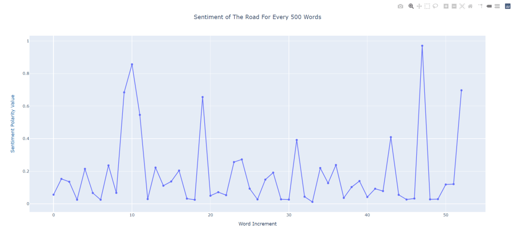
This books a pretty negative one, as to be expected. A wasteland of gray that holds fetus grilling psychos and a bunch of death isn’t exactly a welcome one. We see a couple of spikes in positivity in sentiment throughout, which does seem to make sense. Throughout the novel, the father and son duo find some food, find some water, and they rejoice. The sudden crashes also seem quite logical, as McCarthy can’t let us be all too happy and almost immediately, the duo encounter trouble. Furthermore, the spikes in the end and the final positive sentiment also makes a ton of sense.

Unfortunately, logic does tend to go out the door for a lot of these sentiment polarities. We take a look at Dune (1965) by Frank Herbert:

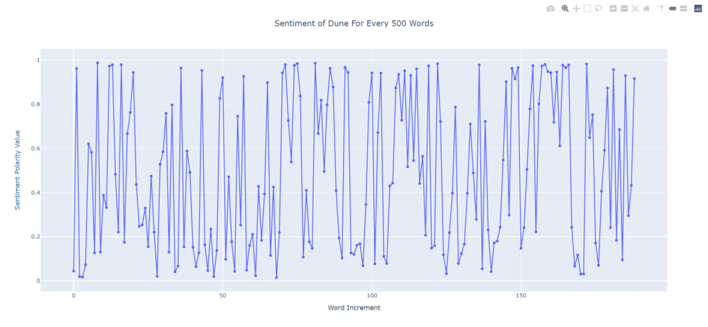
This thing is a chaotic mess. It oscillates up in down, and looks to be quite bimodal, possessing extreme positivity and then extreme negativity in a back and forth manner. I’ll probably give Dune another skim just to see if our classifier is wigging out or if it really is this erratic. For a couple of the works in our data-set, a similar manner of oscillation can be found. Not a great look.

Now for the more meaty bit: The overall average sentiment per era of time. Will there be any consistency? Will it just be another scatter messed? Let’s take a look at this box plot:

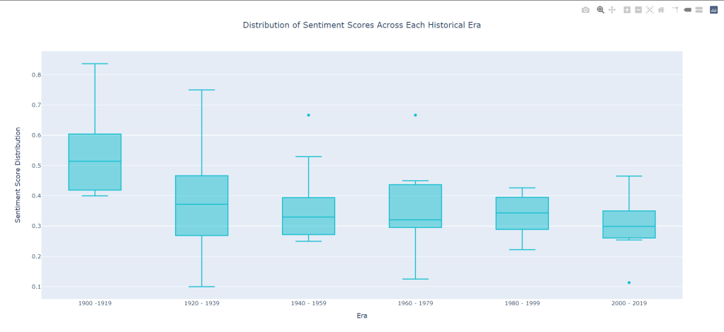
This time we do see a slight relationship. Average sentiment in the earlier eras start out high and gradually dip down and down and down until we bottom out at around 0.3 for the 2000 – 2019s. As we eek forwards in time, we also see our upper and lower fence becoming more tightly packed to our median value (minus that little outlier) so that’s always good to see. Furthermore, There seems to be some sort of relationship. Perhaps the strong dip in sentiment from 1900 – 1919 is due to some real depressing stuff happening (maybe a World War?). Perhaps it is simply due to science fiction becoming more fleshed out and based in social commentary as the genre developed (it was still in an infantile state during that first period). Its all up to speculation.

However, one thing is for sure: These results still aren’t useable. We simply do not have enough books in the data-set. In order to truly be ale to plot an accurate representation, we need some more novels. Some back-stepping is in order before we can truly come to any sort of conclusion. Back to the data-collection-board it is.