Tai Xiang's Random Projects

Moving on from that shoddy first model of voted classifiers, we come about to what is all the rage nowadays: a deep learning model! I had the plan all laid out in my head: Toss a bunch of data into this guy, let him connect the dots, and come out with a trained model that is perfectly accurate and is totally flawless. A plan that could not possibly go wrong.

So how do you train a deep learning model with text? These things usually supposed to take in a bunch of matrices that are composed of numbers right?

Right. In order for our model to make sense of its inputs, we have to convert all of our training set words into individual numbers. We do this by creating a dictionary of numbers that map to individual words. This can look something like this: {(Dog : 1), (Cat : 2), (I : 3), (Walk : 4), (Took : 5), (The : 6), (For : 7), (Walk : 8), (A : 9)}. The string “I took the dog for a walk” would look like this: [3, 5, 6, 1, 7, 9, 8].

We then create matrices out of these numbers and feed them to our model to train on. Furthermore, since our model must take in matrices of the same dimensions, we designate a constant matrix length. We pad reviews that are over this lengths with 0s, and we truncate those that are too large. After this process, a piece of training data will look like this: Basically a bunch of 0s and other numbers that represent words.

[ 0 0 0 0 0 0 0 0 0 0 0 0 0 0 0 0 0 0 0 0 0 0 0 0 0 0 0 0 0 0 0 0 0 0 0 0 0 0 0 0 0 0 0 0 0 0 0 0 0 0 0 0 0 0 0 0 0 0 0 0 0 0 0 0 1 14 22 3443 6 176 7 5063 88 12 2679 23 1310 5 109 943 4 114 9 55 606 5 111 7 4 139 193 273 23 4 172 270 11 7216 10626 4 8463 2801 109 1603 21 4 22 3861 8 6 1193 1330 10 10 4 105 987 35 841 16873 19 861 1074 5 1987 17975 45 55 221 15 670 5304 526 14 1069 4 405 5 2438 7 27 85 108 131 4 5045 5304 3884 405 9 3523 133 5 50 13 104 51 66 166 14 22 157 9 4 530 239 34 8463 2801 45 407 31 7 41 3778 105 21 59 299 12 38 950 5 4521 15 45 629 488 2733 127 6 52 292 17 4 6936 185 132 1988 5304 1799 488 2693 47 6 392 173 4 21686 4378 270 2352 4 1500 7 4 65 55 73 11 346 14 20 9 6 976 2078 7 5293 861 12746 5 4182 30 3127 23651 56 4 841 5 990 692 8 4 1669 398 229 10 10 13 2822 670 5304 14 9 31 7 27 111 108 15 2033 19 7836 1429 875 551 14 22 9 1193 21 45 4829 5 45 252 8 12508 6 565 921 3639 39 4 529 48 25 181 8 67 35 1732 22 49 238 60 135 1162 14 9 290 4 58 10 10 472 45 55 878 8 169 11 374 5687 25 203 28 8 818 12 125 4 3077]

So the first burn went quite smoothly. I used the preloaded Keras IMDB data-set, easily imported into Python. This data-set already has all of the words of the reviews converted to integers that we can directly feed to the machine learning model. All we had to do was pad the reviews to our liking and feed them to our model. Using Keras some more, I created the model and went through a couple runs. Here’s how it looks:

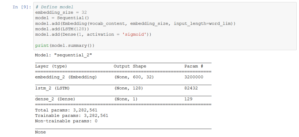
Out of the various deep learning models I had tested, it seem LSTM performed the best for our purposes. An LSTM, or Long Short Term Memory network is a type of recurrent neural network that is capable of learning long-term dependencies. Now what does this mean? Well, as humans with our biological brain and our biological body, we are very much different from the bits of numbers and letters and strings these models are made up of. When we do something – whether it be a task as mundane as brushing our teeth, or drinking water – we utilize our past experiences to optimize how we do these things. Perhaps when we drink water form that bottle with the really big lip, we don’t tilt it as much as the smaller one. Perhaps when we brush our teeth, we make sure to only fill our cup halfway as that is exact amount of water we have determined we need over those years and years (hopefully) of teeth brushing.

Oftentimes, certain models are not capable of this. If we gave some model a toothbrush and let it go at the difficult task of brushing its teeth, it would always fill its cup to the maximal amount because it must start from scratch every single time it performs the task. It isn’t the sharpest tool in the shed, but it sure is persistent. However, we don’t value persistence as much as we value results. So from here, the RNN, or recurrent neural network, steps in.

A recurrent neural network is a little smarter than our run of the mill model. When the gaps between information is small, its little brain can retain that past experience and prevent it from repeating the errors of its ways. If our RNN brushed its teeth yesterday and realized that one full cup of water was too much for rinsing, it’ll only fill three quarter cups the next time. Its retaining information.

However, the RNN starts to struggle when there are bigger gaps between performance of these tasks. Say the last time the RNN brushed its teeth was five days ago (uh oh). When it goes to brush its teeth again, its already forgotten that a whole cup of water was too much. The RNN can no longer piece together these bits of experience after too much time has elapsed. From here, the LSTM steps in.

Even if the last time the LSTM brushed its teeth was five days ago, when it goes back and repeats that task, it’ll remember to only fill its water cup three quarters of the way. It is able to accomplish this astonishing feat through an altered architecture that makes use of multiple interacting layers, forget gates, input gates, and a whole jumble of math and architecture designations. This guy is a little smarter, and thus perhaps when classifying texts, it is able to utilize these past ‘experiences’ to help increase accuracy. Say for instance the LSTM takes in this phrase: “I have a dog. It is a German Shepherd.” The explanation of a dog implies there is likelihood the following phrase will be what breed the dog is. When applying this later to a phrase such as “I have a dog. It is a Golden Retriever.” The LSTM can apply that prior experience to this new input.

Now that we are out of the weeds of fancy deep learning talk, lets take a look at the results of our runs:

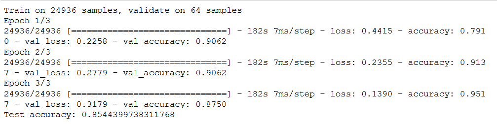
Everything looks pretty good, right? The test accuracy we have after running this model on another 25,000 reviews looks pretty decent at 85.44%. That wasn’t too hard either. Keras’ predesignated bits of deep-learning architecture are pretty easy to use.

And thus the hiccups begin.

Now that we have the model, naturally we want to test it on our own data. However, since the keras imdb dataset is a pre-converted data-set, I did not actually have the dictionary that mapped ints to words, and thus I could not find a way to actually convert my own text data to integers that fit our Keras model. What integer was the word “I” mapped to? What about “Them” or “Hotdog”? I had no clue.

Finally, after a time consuming wild goose chase of documentation, stackoverflow threads, and various forums, a goose came about. Keras did indeed have a dictionary loaded in along the IMDB data-set:

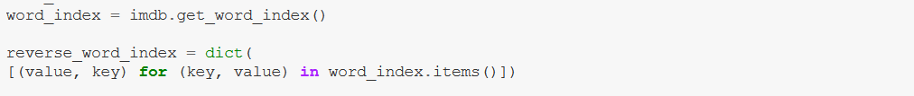
imdb.get_word_index is the designated dictionary. Using that, we can now convert our text into the same integers our training data was keyed to. Perfect. We can begin testing some data.

Now, while I am in this lull of false security, the machines strike another blow: A couple more hiccups (aka mistakes on my part) come about.

The first issue is due to the nature of the IMDB data-set. Since it is a bunch of pre-converted integers, there is no way for us to run any pre-processing/cleaning methods on the data beforehand. Checking the imdb.get_word_index dictionary, I noticed all of the stopwords and whatnot were still in text. Furthermore, all of the words were not lemmatized, so a variety of different word forms were in the dictionary. These factors complicate the dictionary and expand the vocabulary size which in turn make life harder for our poor model that already must do so much work. We don’t need swimming, swam, swum, and swimmer all in the dictionary, we just need swim. These pre-processing methods allow our models to be more accurate. The Keras data-set did not make this easy.

The second issue is of course due to my own negligence (a classic). When feeding the training data-set into the model, I did not shuffle the data. The IMDB data-set is preset to be a perfect 50/50 split, with the first 12500 reviews being all positive and the second 12500 reviews being all negative. Compounding this issue, the testing set is also a perfect 50/50 split. This is not something we want to feed into our model if we want it to turn out well.

So I instead turned to training an entirely new model with a different set of data that was just a bunch of text. This was also a data-set of IMDB movie reviews, 50,000 in total (maybe it was the same as the Keras one, who knows). This time, I pre-processed the data with a couple of old friends and some new ones we made along the way. It looks something like this:

def preprocess_reviews(reviews):
    lemmatizer = WordNetLemmatizer()
    tokens = word_tokenize(reviews)
    # convert to lower case
    tokens = [w.lower() for w in tokens]
    # remove punctuation
    table = str.maketrans('', '', string.punctuation)
    stripped = [w.translate(table) for w in tokens]
    # remove remaining non-alphabetic words
    words = [word for word in stripped if word.isalpha()]
    stop_words = set(stopwords.words('english')+list(punctuation))
    cleaned = [w for w in words if w not in stop_words]
    super_clean = [lemmatizer.lemmatize(word) for word in cleaned]
    return super_clean

Pretty similar to our old NLTK cleaning definition (spoilers: Its copy-pasted). After cleaning our training data, we no longer have stop words and all of our word forms are lemmatized. Now, we’ve got to create our own dictionary of word-to-integer mappings (that we don’t need to scour the internet to find). This is how it looks:

from collections import Counter

counts = Counter()
for line in cleaned_reviews_train:
    nums = Counter(line)
    counts = counts + nums
counts = Counter(el for el in counts.elements() if counts[el] >= 2)
vocab = sorted(counts, key=counts.get, reverse=True)
vocab_to_int = {word: ii for ii, word in enumerate(vocab, 1)}
pickle_out = open("vocab_to_word_dict", "wb")
pickle.dump(vocab_to_int, pickle_out)
pickle_out.close()

After creating our dictionary of words, we remove all words that appear two or less times with this bit of code: *counts = Counter(el for el in counts.elements() if counts[el] >= 2)*. This way, we don’t get any words that are too obscure in our dictionary. (Trust me, some of them were real obscure. “Yaaaaaaaawwwwwwwwwnnnnn” appeared in one of the reviews). We convert our training data into integers, pad it, and get ready for training. Now, we just create a model like we did last time and run it with our training data (except we actually shuffle our training data). We validate it on 1000 samples split away from our training data. Its looking pretty good.

Now with all those wrinkles out of the way, we want to see what combination of architectures gives us the best results. How many dense layers do we want? How many epochs do we need? How many nodes do we want? We want to try out a bunch of these so we can pick the one with the best accuracy. To do this, we use some loops and train a bunch of different models. Here’s how that looks:

dense_layers = [1,2,3]
layer_sizes = [32,64,100,128]
embedding_sizes = [32, 64, 128]

for dense_layer in dense_layers:
    for layer_size in layer_sizes:
        for embedding_size in embedding_sizes:
            NAME = "no_keras-{}-embed-{}-nodes-{}-dense-{}".format(embedding_size,layer_size, dense_layer, int(time.time()))
            print(NAME)
            model = Sequential()
            model.add(Embedding(vocab_content, embedding_size, input_length=word_lim))
            model.add(LSTM(layer_size))
            for _ in range(dense_layer):
                model.add(Dense(layer_size))
                model.add(Activation('sigmoid'))
            model.add(Dense(1, activation = 'sigmoid'))
            
            tensorboard = TensorBoard(log_dir="logs/{}".format(NAME))

            model.compile(loss='binary_crossentropy',
                          optimizer='adam',
                          metrics=['accuracy'],
                          )
            batch_size = 64
            num_epochs = 4
            
            X_valid, y_valid = X_train[:batch_size], y_train[:batch_size]
            X_train2, y_train2 = X_train[batch_size:], y_train[batch_size:]

            model.fit(X_train2, y_train2,
                      validation_data=(X_valid, y_valid),
                      batch_size=batch_size,
                      epochs=num_epochs,
                      callbacks=[tensorboard])
            
            scores = model.evaluate(test, labels_test, verbose=0)
            print(NAME + 'Test accuracy:', scores[1])

Through this block of code, we can try out different combinations of dense layers, LSTM layer sizes, and embedding sizes. I also narrowed in on 3 epochs as being optimal, and thus I run these guys all with 3 epochs. We link it all to tensorboard so we can see some tidy graphs. This is an example of what the whole convoluted bunch look like after running them. In this case, we show the progression of accuracy through each epoch:

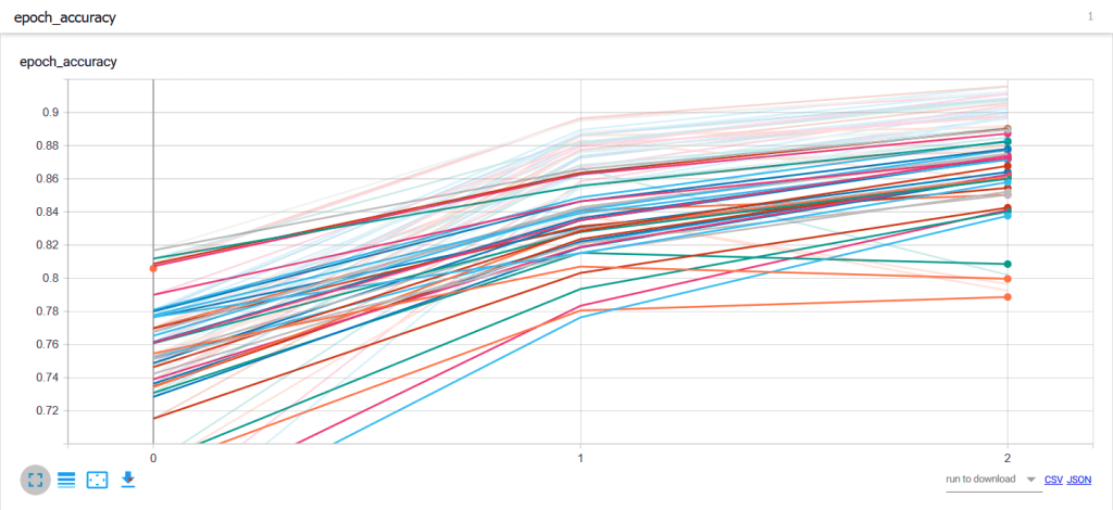
After these runs, we try to narrow in on which combination of factors lead to the best model. That model becomes the chosen one and we use it to classify our text.

An advantage of this new deep learning model is that it is capable of detecting sarcasm. When we run the phrase “Great. Its raining again. I can’t get enough of the rain. This day can’t get any better.”, our classifier deems this to be of negative sentiment. Instead of simply viewing the representation as a bag of words, this deep learning model is able to form relationships and detect subtleties in how these phrases are organized. It is much more powerful than the previous model we designated using a host of NLTK classifiers, and it is also more accurate. However, I think I did pull out more hair building this one in comparison to the NLTK voted classifier model. You win some, you lose some I guess.

Now, all we gotta do is plug our books into the pre-processing flow and feed them through our saved model. Lets see how we do this time. Hopefully the data is a bit more interesting.